CFD Surrogate Studio — User Manual

A surrogate-model web app that predicts stirred-tank, shake-flask and rocking-bag flow fields, power draw, mass/heat transfer and solids suspension in seconds — no CFD license, no meshing, no waiting.
Surrogate CFD Stirred tank · Shake flask · Wave bag 23 impeller types Np · Fl · kLa · Power Beginner-friendly

1What is CFD Surrogate Studio?

It is a fast reduced-order ("surrogate") model of a mixing vessel. Instead of solving the full Navier–Stokes equations on a million-cell mesh, it uses engineering correlations (power number, flow number, Metzner–Otto shear, Zwietering suspension, etc.) plus a jet-based reduced field solver to estimate the velocity, shear, power, kLa, heat and solids behaviour of your vessel.

When to use it

Early design, "what-if" screening, scale-up sanity checks, teaching, and quick checks of power / tip speed / flooding before you commit to a full CFD or experiment.

What you get

Flow-field plots, turbulence & shear, power & regime, gas mass transfer (kLa/OTR), heat transfer, solids suspension, scale-up rules and an auto-generated report.

What it is NOT

A high-fidelity CFD solver. It ranks designs and explains trends; it is not a substitute for validated CFD or experimental confirmation on a final, regulated design.

Three platforms, one tool: stirred (tanks with impellers/baffles), shaken (orbital shake flasks / OSB) and rocked (wave/rocking bags). Geometry shapes the drawings: round = cylinder, square = PETG box, pillow = wave bag.

23-step quick start

1
Set up the vessel (left sidebar). Pick platform → container family → size preset, then tweak geometry, liquid, impeller and speed.
2
Click ▶ Run at the bottom of the sidebar. The analysis takes a few seconds and the result tabs appear.
3
Read the results using the horizontal tab bar: Overview → Flow field → Turbulence & shear → Power & regime → … → Report. Red warnings in Overview tell you exactly what to fix.
Everything is editable. A preset only seeds the dimensions once — you can type any odd size (e.g. 655 L) afterwards.

3Input guide (sidebar)

The sidebar is organised as six numbered steps. Ranges below are the exact limits enforced in the app.

Step 1 · Platform

Choose stirred, shaken or rocked. This decides which container families, impellers and result tabs are available.

Step 2 · Container family + geometry

Step 3 · Size — ONE method

Pick either "Type dimensions" or "Type target liquid litres" (e.g. 655 L). You never enter the same quantity twice.

Step 4 · Liquid property

Step 5 · Impeller

Step 6 · Speed & process context

Tip: The Overview tab runs "engineering checks" — flooding, Njs (just-suspended speed), tip-speed cell damage, torque vs stir-plate limit, unfavourable swirl. Fix what it flags before trusting the numbers.

4Blade-type atlas (23 impellers)

Every impeller is characterised by its turbulent power number Np∞, laminar asymptote Kp (Np·Re limit), primary flow number Fl, and Metzner–Otto shear constant ks. The family cards below use clean 3D product-style renders for realism; the close-clearance family uses a schematic because anchor/ribbon geometry is clearer drawn than rendered.

Radial Mixed flow Axial Close-clearance Disperser
RADIAL

Radial-flow turbines — discharge straight out, then split up & down
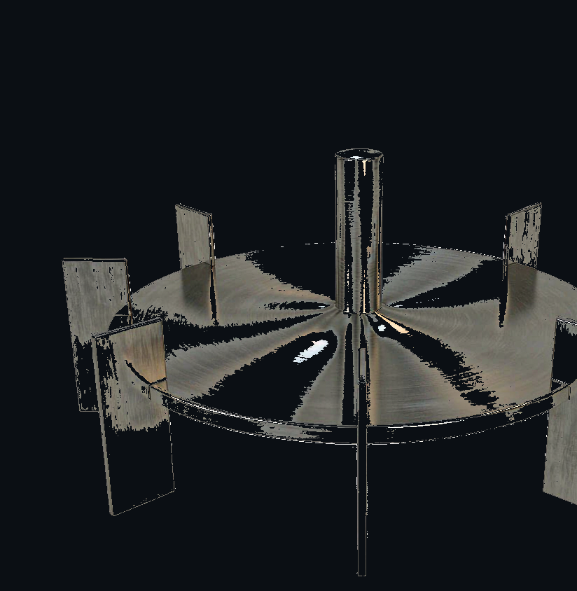
Rushton 6-blade disc turbine: a horizontal disc with six flat vertical rectangular blades mounted around the rim, viewed from above

Blades sit on a disc and throw liquid radially outward, creating two circulation loops (up the wall, down the centre, or vice-versa). Highest shear at the blade tips — great for gas dispersion, harsher on shear-sensitive cells.

  • Rushton DT-6 — the classic 6-blade disc turbine, Np≈5.0 (Bates et al. 1963).
  • CD-6 / BT-6 / Scaba 6SRGT — concave / hollow blades; better gas handling and kLa efficiency at lower Np.
  • Flat paddle (2-blade) — large-D/T, common in glass vessels & DS bottles.
MIXED

Mixed-flow — pitched blades, mostly downward axial with radial component
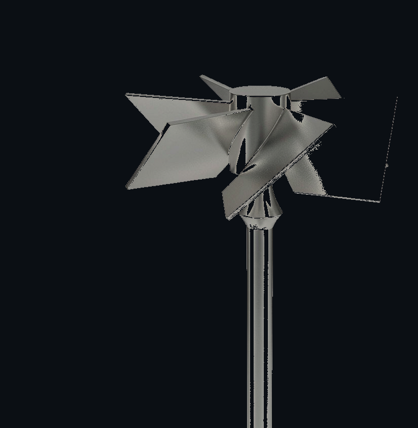
Pitched blade turbine with six flat blades tilted at 45 degrees on a central hub, a typical mixed-flow impeller

Pitched-blade turbines (PBT) blend axial and radial flow. 4×45° and 6×45° are axial-dominant workhorses for blending and moderate gas handling. Magnetic stir bars (egg, cylindrical, octagonal, cross, floating, pivot-ring) are up-pumping mixed-flow devices for bottles and shake-style vessels.

  • PBT 4×45°: Np∞ 1.60; PBT 6×45°: Np∞ 1.85.
  • Stir bars: Np∞ 0.70–1.15; cross strongest, floating weakest. Effective hydraulic D ≈ 0.7× bar length.
AXIAL

Axial-flow hydrofoils & propellers — strong top-to-bottom pumping, low shear
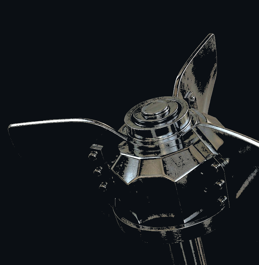
Three-blade hydrofoil axial impeller with swept curved blades, designed for gentle top-to-bottom pumping

High-efficiency, low-power-number blades that push liquid axially (top-to-bottom), giving excellent bulk blending and gentle shear — ideal for cell cultures. Propellers and low-pitch PBTs also fall here.

  • A310 / HE-3 hydrofoils: Np∞ ≈ 0.30 — the efficiency champions.
  • Maxflo WSE: up-pumping, Np∞ 0.48.
  • Marine propellers (pitch 1.0 / 1.5): Np∞ 0.32 / 0.55.
  • PBT 4×30°: Np∞ 0.95, more axial than the 45° version.
CLOSE-CLEARANCE

Anchor & helical ribbon — hug the wall, dominate in laminar / high-viscosity duties

anchor / helical ribbon · tangential sweep

Close-clearance agitators sit near the wall to scrape and circulate highly viscous fluids. High Kp (laminar power asymptote) and high ks (shear). Used for heat-transfer and laminar blending.

  • Anchor (D/T≈0.9): Np∞ 0.55, Kp 280, ks 22.
  • Helical ribbon (D/T≈0.95, pitch 1): Np∞ 0.38, Kp 340, ks 30 — laminar blending workhorse.
DISPERSER

Sawtooth (Cowles) disperser — extreme local shear for emulsification & deagglomeration
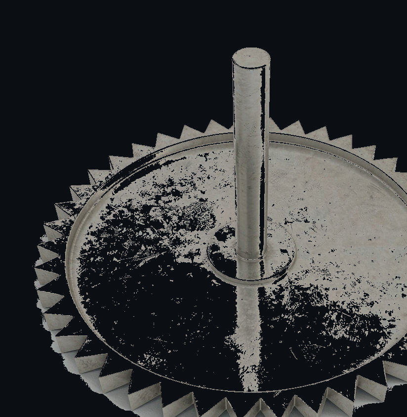
Cowles sawtooth disperser: a flat circular disc with sharp triangular teeth around the rim, used for extreme local shear

A toothed disc that generates intense localized dissipation for dispersing solids into liquids and making fine emulsions. Very low flow number, very high local shear — not for bulk blending.

  • Cowles sawtooth: Np∞ 0.17, Kp 145, Fl 0.22, ks 14.

Full impeller data table

ImpellerFamilyPumping Np∞KpFlksNotes
Rushton DT-6 (6-blade disc)radialradial5.001100.7511.5Classic radial turbine; flat blades on disc.
Concave CD-6 (Smith)radialradial3.05900.7611.0Semi-circular blades; high gas-handling kLa.
Concave BT-6 (backward curved)radialradial2.55800.7210.5Backward-curved concave blade.
Scaba 6SRGT (hollow blade)radialradial3.20950.7311.0Hollow-blade radial gas disperser.
Flat paddle 2-blade (w/D=0.25)radialradial1.75580.6511.0Large-D/T; glass vessels & DS bottles.
Pitched blade 4×45°mixeddown1.60620.7911.0Axial-dominant mixed flow.
Pitched blade 6×45°mixeddown1.85700.8311.5Axial flow number ≈0.75.
Stir bar — egg / ellipticalmixedup0.85550.5511.0Self-centring in round bottles; lab default.
Stir bar — cylindricalmixedup0.80520.5210.5Plain cylinder; spins out first at high N.
Stir bar — octagonalmixedup0.95580.5811.5Facets add shear/pumping vs cylinder.
Stir bar — cross / plusmixedup1.15640.6212.0Highest pumping of the bars; DS pooling bottles.
Stir bar — floating / bobbingmixedup0.70500.4810.0Rides near surface; weak bottom turnover.
Stir bar — pivot-ringmixedup0.90560.5611.0High-grip; higher coupling limit.
Pitched blade 4×30°axialdown0.95520.6810.5More axial than the 45° version.
Lightnin A310 hydrofoil (3-blade)axialdown0.30420.5610.0High-efficiency solid-set; low Po/Fl.
Chemineer HE-3 hydrofoilaxialdown0.30440.5310.0High-efficiency hydrofoil.
Maxflo WSE hydrofoil (4-blade)axialup0.48480.6310.5Up-pumping axial hydrofoil.
Marine propeller pitch 1.0axialdown0.32410.5010.0Classic 3-blade marine propeller.
Marine propeller pitch 1.5 (SC-3)axialdown0.55460.8210.5Higher pitch → more pumping.
Anchor (D/T≈0.9)closetangential0.552800.3022.0Heat-transfer duty; Np T/D-dependent.
Helical ribbon (D/T≈0.95, p=1)closetangential0.383400.2530.0Laminar blending workhorse.
Sawtooth disperser (Cowles)disperserradial0.171450.2214.0Ultra-high shear; extreme local dissipation.

Np∞ = turbulent power number at standard D/T=1/3, w/D=1/5. Kp = laminar Np·Re asymptote. Fl = primary flow number. ks = Metzner–Otto average shear-rate constant. All are editable in the app's Advanced panel.

5Vessel preset library

Presets seed the geometry; everything stays editable. "Deq" is the area-equivalent diameter used by the correlations (square PETG bottles and wave bags are screened on Deq).

PresetModeFootprintH [m]FillBaffledNotes
Ambr-type mini bioreactor 250 mLstirredØ68 mm0.120.65yes (4)Glass, full jacket.
Glass STR 2 LstirredØ130 mm0.210.72yesDished bottom.
Glass STR 10 LstirredØ210 mm0.310.75yesDished bottom.
Pilot STR 50 L (316L)stirredØ350 mm0.520.75yesStainless, dished.
Production STR 2000 L (316L)stirredØ1.15 m2.000.75yesBottom-jacketed, dished.
Single-use stirred 200 LstirredØ550 mm0.850.70noFilm wall; unbaffled swirl expected.
DS bottle 2 L (stir bar)stirredØ135 mm0.240.65noCircular, flat, stir bar.
DS bottle 10 L (stir bar)stirredØ230 mm0.360.70noCircular, flat, stir bar.
PETG bottle 500 mL (square)stirred70×70 mm0.170.60noDeq≈79 mm (screening).
Shake flask 250 mLshakenØ83 mm0.130.18noOrbital shaker.
OSB 3 L / 50 L tubeshakenØ120 / 340 mm0.32 / 0.620.28 / 0.25noOrbital shaken bioreactor.
Wave / rocking bag 20 Lrocked300×500 mm0.220.45noPillow bag on rocking platform.
Mobile vessel 50–1000 LstirredØ394–1070 mm0.51–1.390.80no316L; bottom (flat/dished/conical) selectable.
Custom geometrystirred—0.300.70optionalType any dimensions you like.

6Liquid / fluid presets

Pick a category then a fluid, or toggle Custom liquid to type density & viscosity directly. Non-Newtonian presets use shear-thinning (power-law) or yield-stress models.

Aqueous buffers & media

Water (purified), WFI, PBS buffer, cell-culture basal medium, CHO fed-batch broth (~20e6 c/mL, μ≈1.15 mPa·s).

Sugar & glycerol solutions

Sucrose 60 Bx, glucose syrup ~70 DS, glycerol 50 wt%, glycerol 99.5% (μ≈945 mPa·s).

Fermentation & microbial

E. coli broth (μ≈2.5 mPa·s), fungal broth (A. niger type, μ≈0.8 Pa·s).

Non-Newtonian & complex

CMC 0.5 / 1.5 wt% (pseudoplastic), xanthan 0.2 wt% (yield-like), kaolin slurry 40 wt%, blood (Casson-like).

Oils

Silicone oil 10 cSt / 100 cSt, light mineral oil.

Other

Ethanol 30 vol%; Custom (type ρ 500–3000 kg/m³, μ 0.01–1e6 mPa·s).

Process-context guideline bands

Selecting a context adds P/V and tip-speed warning bands in the Overview:

ContextP/V band [W/m³]Tip-speed limit [m/s]
Mammalian (CHO / HEK)20 – 802.0
Insect (Sf9)25 – 1202.2
Plant cell10 – 401.2
Microbial (E. coli / yeast)2000 – 120008.0
Filamentous fungi1500 – 80006.0

7Reading the results

After ▶ Run, a horizontal tab bar appears (stirred mode shows all nine; shaken/rocked show Overview only). A red verdict in Overview links you straight to the tab that fixes the problem.

Overview

Tags (platform, shape, fluid, volume, baffling) + engineering checks: flooding, Njs, tip-speed damage, torque vs stir-plate limit, swirl. Start here.

Flow field

Velocity magnitude, vectors and streamlines; radial-profile plots of axial/radial velocity and shear. Open the Virtual tracer t95 expander for blending time (θ95 / t95) and the Agitation duration input — set how long you will actually agitate and it reports the tank homogeneity at that instant (% of virtual probes within ±5% of the fully-mixed target).

Turbulence & shear

Turbulent kinetic energy, dissipation ε, Kolmogorov eddy size η, Metzner–Otto shear rate — key for cell-damage assessment.

Power & regime

Power draw P, P/V, Reynolds number Re, laminar↔turbulent transition, tip speed.

Gas & mass transfer

kLa, OTR vs OUR, flooding/dispersing check, sparge vvm. Shown when sparging is enabled.

Heat transfer

Wall/U coefficient, utility duty, fouling margin. Shown when thermal analysis is enabled.

Solids

Just-suspended speed Njs, suspension homogeneity, settling vs pumping. Shown when solids are present.

Scale-up

Rules (constant P/V, tip speed, ε, Njs…) applied between your vessel and a target scale.

Report

Auto-generated summary of inputs, outputs and warnings — copy or export for records.

8Worked example — 1000 L CHO fed-batch fermenter

1
Platform: stirred. Family: Cylindrical STR (round glass/SS). Preset: Production STR 2000 L, then set working volume to 1000 L (litres mode solves Ht & fill).
2
Liquid: CHO fed-batch broth (ρ≈1015 kg/m³, μ≈1.15 mPa·s). Context: mammalian (CHO/HEK) → P/V band 20–80 W/m³, tip ≤2.0 m/s.
3
Impeller: 2× Rushton DT-6 (or 1× Rushton + 1× A310 for lower shear), D ≤ 0.95·T, lower impeller near the bottom, upper impeller in the upper loop.
4
Speed: set rpm so P/V stays in 20–80 W/m³ and tip speed ≤2.0 m/s. Enable sparging (vvm) for kLa/OTR; check Gas & mass transfer vs OUR.
5
Read: Overview flags any flooding/tip-speed issue; Turbulence & shear confirms Kolmogorov eddy η is large vs cell size; Gas & mass transfer confirms OTR > OUR.
This screening tells you whether the geometry/impeller/speed is in a safe, productive regime before you build or run the real vessel.

9Theory, formulas & assumptions

Every number in CFD Surrogate Studio comes from closed-form correlations and a reduced-order (surrogate) flow field — not a mesh-resolved CFD solve. This section lists the exact equations so you can audit, reproduce, or override them. All coefficients (k≈5.9, ks, Po, Fl, van't Riet a…) are editable in the app's Advanced panel.

1Reynolds number & flow regime

Shaft speed is converted to revolutions per second N = rpm / 60. The impeller Reynolds number sets the regime:

Re = ρ · N · D² / μ

For non-Newtonian broths the apparent viscosity is evaluated at the Metzner–Otto mean shear rate γ̇ = ks · N (ks ≈ 11.5 for a Rushton), so μ = μapp(γ̇, T) feeds back into Re. Regime bands: Re < 10 laminar, 10–1000 transitional, > 1000 turbulent.

2Power, tip speed & Froude

Power number per impeller follows a generalised laminar→turbulent curve (Bates-style blending) into the turbulent plateau Np∞:

Np(Re) = ( (Kp / Re)c + Np∞c )1/c

Power draw, intensity and the two dimensionless speeds then follow directly:

P = Np · ρ · N³ · D⁵  ·  P/V  ·  ε̄ = P / (ρ·V)  ·  utip = π·N·D  ·  Fr = N²·D / g

Multiple impellers are de-rated when stacked closer than ≈1 D (interaction factor 0.55–1.0). Froude is used for the vortex-depth correction and the unbaffled-vessel warning (Fr > 0.2 → central vortex).

3Circulation & blend time (homogeneity)

Each impeller pumps a volumetric flow and the bulk turns over in a circulation time:

Q = Fl · N · D³  ·  τcirc = V / (Q · 2.2)  (2.2 = entrained-flow factor)

Blending time uses the Grenville & Nienow correlation. Turbulent:

N · θ95 = k · Po−1/3 · (T/D)²   with k ≈ 5.9

Laminar extension (Grenville & Tilton) and a smooth log(Re) blend in the transitional range:

N · θ95,lam = 183 · Po−1/3 · (T/D)²   →   θ95 ∝ 1/N

Two physical corrections: (a) a floor θ95 ≥ τcirc (you cannot blend faster than one turnover), and (b) a multi-impeller de-rating θ95 /= nimp0.25. Target windows default to 60 s (mammalian) / 30 s (microbial).

4Virtual tracer t95 (the time-to-mix model)

The "Agitation duration" input and the t95 verdict come from a reduced-order compartment model run on the developed flow. Each virtual probe relaxes toward the fully-mixed concentration as a first-order process:

C/C∞(t) = 1 − A · exp(−ki · t)

where the local rate ki is set by the local |U|/shear field (dead corners mix ≈20× slower than the impeller jet) and the whole set is calibrated so the median probe t95 equals the Grenville θ95. A probe is "mixed" once its curve stays inside the ±5% band:

t95 = first t with 0.95 ≤ C/C∞ ≤ 1.05 (and stays)

The reported "Homogeneity at chosen t" is the percentage of virtual probes whose C/C∞ lies inside that same ±5% band at the instant you specify — i.e. the fraction of the tank homogeneous after your actual agitation time. The PDE-beta variant transports mass between cells on a coarse r–z grid (max-t95 ≈ 2× θ95, unpinned) for an audit-style cross-check; the OpenFOAM export gives fully mesh-resolved t95.

5Turbulence micro-scales (shear / cell damage)

The surrogate reconstructs turbulence from the velocity gradients of the reduced field. Fluctuating velocity uses a Prandtl mixing length:

u′ = ℓm · γ̇,   ℓm = 0.41·dwall (clipped to 0.002–0.09·T)

Turbulent kinetic energy, dissipation and the Kolmogorov microscale:

k = 1.5·u′²  ·  ε = 0.164·k1.5 / ℓm  ·  η = (ν³ / ε)1/4

Impeller-swept zones are floored at 6·ε̄ to reflect localised dissipation. The mammalian shear check uses η ≥ 25 µm pass, 15–25 marginal, < 15 fail (eddy ≈ cell size). Mean strain rate γ̇ = √(2·S:S).

6Gas mass transfer

Gassed power uses Michel–Miller (1962); kLa uses van't Riet (1979), steady-state, valid to ≈2600 W/m³:

kLa = a · (Pg/V)e1 · vse2 · exp(0.024·(T − 20))

Coalescing broth: a = 0.026, e1 = 0.4, e2 = 0.5; non-coalescing: a = 0.002, e1 = 0.7, e2 = 0.2. OTR (at the DO set-point) is compared against OUR to flag under-aeration; Nienow flooding correlation reports FLOODED / Loading / Dispersed (flooded = critical fail).

7Solids suspension

Just-suspended speed uses the Zwietering correlation Njs (critical fail if N < Njs); a homogeneous distribution needs roughly 1.3·Njs. A quiescent single-particle settling velocity Vt flags fast settlers (Vt > Q/A) but does not replace the Njs criterion.

8The 8-check verdict rule

The traffic-light in Overview answers "will this batch mix at this speed?": any critical fail (flooded / N < Njs / OTR < 0.5·OUR) or ≥2 fails → red; 1 fail or ≥3 marginals → amber; 1–2 marginals → amber "mostly mixed"; else green. The rough speed to hit a target blend time is rpm_hint ≈ N · θ / θ_target.

These are engineering screening correlations — excellent for ranking geometries, speeds and fluids and for catching unsafe regimes before you build or run the real vessel. They are not a substitute for mesh-resolved CFD or experimental confirmation on regulated final designs.

10Model limitations & best practice

Surrogate, not CFD

Correlation + jet-based reduced field. Great for ranking and trends; not a mesh-resolved solution. Confirm final regulated designs experimentally.

Screening for non-round shapes

Square PETG bottles and wave bags run on area-equivalent diameter Deq. Ranking is preserved, but absolute values are screening-level.

Stir-bar slip

Magnetic bars can slip/stall above the plate coupling limit — check the Overview torque warning, especially for viscous or large bars.

Single-phase assumptions

Gas/heat/solids modules need their toggles on and reasonable inputs; they are estimates, not multiphase CFD.

Best practice: Always read the Overview engineering checks first. Treat the tool as a fast "what-if" engine and a sanity checker — pair it with experiments for final sign-off.